The error ellipse (probability ellipse) is an ellipse illustrating the variance of a two-dimensional normal distribution.
From the variance-covariance matrix of the normal distribution, the formula for the ellipse can be calculated to cover any range.
This article explains how to calculate the ellipse using Python drawing in Matplotlib as an example.
Error ellipse(Probability ellipse)
Consider data that are normally distributed in the two-dimensional space of \(x,y\).
An error ellipse (probability ellipse) is an elliptical representation of the range over which the data are scattered from the centre (mean) of the normal distribution.
The size of the error ellipse (probability ellipse) is determined by what percentage of the total data is drawn to be covered.
The formula for the ellipse is then found by calculating the diagonalisation of the variance-covariance matrix of the normal distribution.
matplotlib.patches.Ellipse
To draw ellipses in Python, use matplotlib.patches.Ellipse.
This function mainly requires the following parameters to be specified, so you need to calculate these values from the distribution formula.
| parameter | content |
|---|---|
| xy | Ellipse centre coordinates |
| width | Length of the horizontal axis of the ellipse (this time the major axis) |
| height | Length of the vertical axis of the ellipse (this time the minor axis) |
| angle | Elliptical tilt angle (degree) |
Example
Below is an example calculation, considering a specific distribution.
Calculation.
Draw the error ellipse (probability ellipse) of the two-dimensional normal distribution represented by the mean \(\boldsymbol{\mu}=(8, 12)\) and variance-covariance matrix
$$\boldsymbol{\Sigma}=\begin{pmatrix} \sigma_x^2 & \sigma_{xy} \\ \sigma_{xy} & \sigma_y^2 \end{pmatrix}=\begin{pmatrix} 16 & \sqrt{78} \\ \sqrt{78} & 9 \end{pmatrix}$$
If the variance-covariance matrix is diagonalised, the variance-covariance matrix after diagonalisation can be written as
$$\boldsymbol{\Sigma}'=\begin{pmatrix} \sigma_u^2 & 0 \\ 0 & \sigma_v^2 \end{pmatrix}$$
Here,
$$\sigma_u^2=\frac{(\sigma_x^2+\sigma_y^2)+\sqrt{(\sigma_x^2-\sigma_y^2)^2+4\sigma_{xy}^2}}{2}$$
$$=\frac{(16+9)+\sqrt{(16-9)^2+4\cdot 78}}{2}=44/2=22$$
$$\sigma_v^2=\frac{(\sigma_x^2+\sigma_y^2)-\sqrt{(\sigma_x^2-\sigma_y^2)^2+4\sigma_{xy}^2}}{2}$$
$$=\frac{(16+9)-\sqrt{(16-9)^2+4\cdot 78}}{2}=6/2=3$$
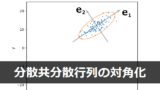
The following article explains in more detail how to diagonalise a variance-covariance matrix.
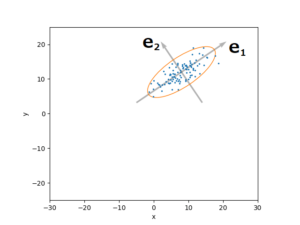
Also, the basis vector corresponding to this diagonalisation is
$$\mathbf{e}_1=\left(1,\frac{\sigma_u^2-\sigma_x^2}{\sigma_{xy}}\right)=\left(1,\frac{22-16}{\sqrt{78}}\right)=\left(1,\frac{6}{\sqrt{78}}\right)$$
$$\mathbf{e}_2=\left(1,\frac{\sigma_v^2-\sigma_x^2}{\sigma_{xy}}\right)=\left(1,\frac{3-16}{\sqrt{78}}\right)=\left(1,-\frac{13}{\sqrt{78}}\right)$$
In the \(u-v\) plane with variable transformation along the basis vector \(\mathbf{e}_1,\mathbf{e}_2\), the expression for the ellipse corresponding to the distribution can be written as
$$\frac{u^2}{\sigma_u^2}+\frac{v^2}{\sigma_v^2}=c^2\tag{1}$$
The variables \(\frac{u}{\sigma_u}\) and \(\frac{v}{\sigma_v}\) follow a standard normal distribution, so their sum of squares \(c^2\) follows a chi-square distribution with 2 degrees of freedom.
Below, the relationship between the cumulative distribution function \(P\) (the proportion of data covered by the ellipse), \(c^2\) and \(c\) in a chi-square distribution with two degrees of freedom is displayed.
| \(P\) | 0.393 | 0.500 | 0.900 | 0.950 | 0.990 |
|---|---|---|---|---|---|
| \(c^2\) | 1.000 | 1.385 | 4.605 | 5.992 | 9.211 |
| \(c\) | 1.000 | 1.177 | 2.146 | 2.448 | 3.035 |
From these, select the values of \(c^2\) and \(c\) that correspond to the range of the distribution you wish to display using the error ellipse (probability ellipse).
In the equation \((1)\), when \(v=0\)
$$\frac{u^2}{\sigma_u^2}=c^2\Leftrightarrow u=\pm c\sigma_u$$
Similarly, when \(u=0\)
$$\frac{v^2}{\sigma_v^2}=c^2\Leftrightarrow v=\pm c\sigma_v$$
Therefore, the lengths of the major radius and minor radius of the ellipse are (csigma_u, csigma_v), respectively.
Therefore, the lengths of the major axis (width) and minor axis (height) of the ellipse are \(2c\sigma_u, 2c\sigma_v\), respectively.
For example, for \(P=0.950\), they are
$$2c\sigma_u=2\cdot 2.448\cdot\sqrt{22}\simeq 22.96$$
$$2c\sigma_v=2\cdot 2.448\cdot\sqrt{3}\simeq 8.480$$
Finally, the angle between the major axis (\(\mathbf{e}_1\)) and the \(x\) axis is determined as the inclination angle of the ellipse.
Because of
$$\mathbf{e}_1=\left(1,\frac{6}{\sqrt{78}}\right)$$
if the angle between this vector and the \(x\) axis is called \(theta\), then
$$\tan{\theta}=\frac{6}{\sqrt{78}}$$
Therefore,
$$\theta=\arctan\left(\frac{6}{\sqrt{78}}\right)\simeq 34.19^\circ$$
(If \(\arctan\) is returned in radians, modify to degrees)
From the above, the parameters of the ellipse are specified this time as follows.
| parameter | content | value |
|---|---|---|
| xy | Ellipse centre coordinates | [8,12] |
| width | Length of the horizontal axis of the ellipse | 22.96 |
| height | Length of the vertical axis of the ellipse | 8.480 |
| angle | Elliptical tilt angle (degree) | 34.19 |
Source code
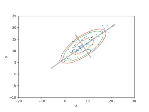
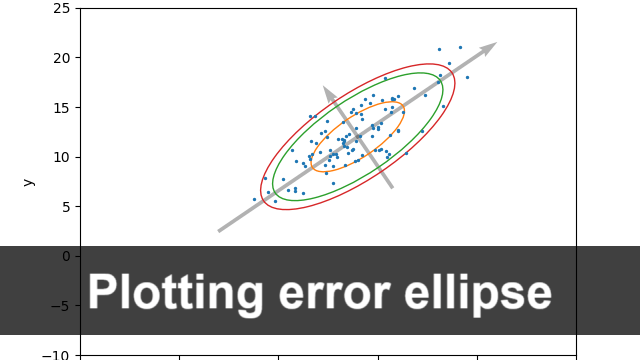
In the code below, the error ellipses (probability ellipses) covering 50% (orange), 90% (green) and 95% (red) of the range are plotted together with the axis of the basis vector.
The width and height for \(P=0.500, P=0.900\) can also be calculated as for \(P=0.950\).
Comments